Vibration testing notes
A vibration test applies a specified mechanical input and measures how an assembly responds. The input, mounting arrangement, duration, and operating condition define the exposure. Inspection and functional checks determine whether the assembly meets the test’s acceptance criteria.
These notes cover sine and random vibration, resonance, measurement, and test setup. The numerical examples are calculated illustrations. They do not represent qualification profiles or measured test results.
1. Fundamental concepts and physical variables
Motion and amplitude
Vibration is motion about an equilibrium position. Free vibration follows an initial disturbance; forced vibration occurs under an applied excitation. Qualification testing applies a defined exposure to a documented configuration. Modal testing measures structural properties, such as natural frequencies and mode shapes. A qualification pass alone does not establish a fatigue life or validate a finite element model.
Displacement x(t) is position relative to a reference. Velocity is dx/dt, and acceleration is d²x/dt². Displacement may be reported in millimetres, velocity in millimetres per second, and acceleration in metres per second squared or g. State whether each amplitude is peak, peak-to-peak, or RMS.
- Peak: the largest magnitude relative to the chosen reference over the measured interval.
- Peak-to-peak: maximum minus minimum. A zero-centred sine wave with peak amplitude X has peak-to-peak amplitude 2X.
- Root mean square (RMS): the square root of the mean of the squared samples. It has the same units as the signal. Acceleration RMS is not an energy measurement.
xRMS = √[(1/N) Σ xn²]
For a zero-mean signal, RMS equals the population standard deviation of those samples. A nonzero mean contributes to RMS, so removing an offset changes the quantity being reported.
Acceleration, velocity, and displacement
For sinusoidal displacement x(t) = X sin(2πft), differentiation gives peak velocity V = 2πfX and peak acceleration A = (2πf)²X. Thus:
X = A / (2πf)²
At constant acceleration, displacement increases as frequency decreases. Low-frequency sine profiles can therefore reach a shaker’s stroke limit at low acceleration levels.
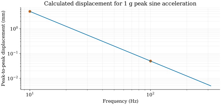
For a pure sine wave, RMS amplitude is peak amplitude divided by √2. That conversion does not specify the peak value of a random waveform.
Input motion and structural response
The acceleration at a mounting interface can differ substantially from the acceleration elsewhere on an assembly. A flexible bracket, circuit board, or housing can amplify motion near a structural mode. An interface sensor measures applied motion at the mounting point; a response sensor measures local motion on the assembly.
A single-degree-of-freedom model represents one mass, spring, and viscous damper. For an applied force F(t), its equation is:
mẍ + cẋ + kx = F(t)
Here m is mass, c is the viscous damping coefficient, k is stiffness, and x is displacement. A dot denotes a derivative with respect to time. The undamped natural frequency and damping ratio are:
fn = √(k/m) / (2π) · ζ = c / (2√(km))
Increasing stiffness raises the natural frequency; increasing mass lowers it. Damping affects the height and width of the response peak. Real assemblies have multiple modes, each with a frequency and deformation pattern. This simplified model describes an isolated mode under linear-response assumptions. Crystal Instruments: structural vibration fundamentals.
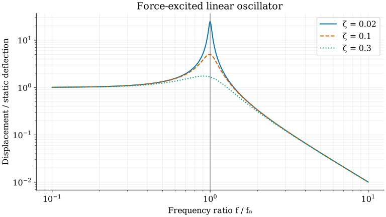
For the figure, the normalized amplitude is 1/√[(1 − r²)² + (2ζr)²], where r = f/fn. A shaker test commonly prescribes base motion instead of applied force. For this same oscillator, the absolute mass-to-base displacement ratio is √[1 + (2ζr)²]/√[(1 − r²)² + (2ζr)²]. Use the amplitude and phase relations for the specified excitation: applied force or base motion.
2. Equipment and closed-loop control
The measurement and drive loop
An electrodynamic shaker produces force through a moving coil in a magnetic field. The amplifier supplies electrical power to the coil. The controller compares measured control-channel motion with the requested profile and adjusts its output. The fixture and test item are part of the mechanical system inside that loop.
Drive path: controller → power amplifier → shaker armature → fixture → test item.
Feedback path: control accelerometer → signal conditioning and digitization → controller.
Shaker systems also need the cooling specified for their operating condition. Amplifier voltage and current, shaker force, velocity, displacement, and payload ratings depend on the selected system. Check the selected system's ratings before running the test. The Modal Shop: shaker systems and accessories.
Accelerometer selection and channel scaling
Integrated electronics piezoelectric (IEPE) accelerometers include signal-conditioning electronics and require a compatible electrical supply. Piezoelectric sensors measure changing acceleration and do not measure steady acceleration at DC. Variable-capacitance sensors can provide DC response for slow motion, tilt, and constant acceleration. The term microelectromechanical systems (MEMS) describes how a sensor is made. Its sensing principle and specified frequency response determine which measurements it can make. Endevco: accelerometer technologies.
Use the calibrated sensitivity for each channel, with matching units. Check the sensor range and acquisition input range against expected peaks. A clipped waveform cannot be recovered by rescaling its plotted spectrum. Sensor bandwidth, mounting, cable routing, and electrical isolation should be checked for the actual installation. Select isolation hardware to suit the sensor mounting and grounding arrangement.
3. Fixture design and pre-test checks
Fixture, sensors, and control
The fixture transfers motion from the shaker to the test item. Its stiffness, mounting interfaces, and resonances affect the applied motion. Control accelerometers are generally placed near the fixture-to-item interfaces, with the control method defined by the test procedure. A response accelerometer measures local motion on the test item. NASA KSC-STD-164, Revision C.
Accelerometer mounting affects usable frequency response. Stud mounting on a suitable surface generally provides a higher mounted resonance than added adhesive or magnetic adapters. Follow the sensor’s mounting instructions and check its mass, orientation, calibration, and range against the measurement requirements. PCB Piezotronics: accelerometer mounting.
A control channel within tolerance does not prove that every point on the assembly received the same input. The test record should identify the channels used for control, response monitoring, and limits.
Fixture stiffness and moving mass
Check fixture strength and dynamic response separately. A static strength calculation does not establish the response across the test band. Fixture flexibility can produce local amplification, phase differences, and cross-axis motion. Motion can differ between attachment points.
Fixture mass and stiffness affect its natural frequencies. Added moving mass increases the force needed for a given rigid-body acceleration. Use F = ma for a preliminary rigid-body force calculation, then check resonant response and the shaker's capability across the test band.
Fixture materials and specific stiffness
Specific stiffness, or specific modulus, is Young’s modulus E divided by density ρ. Young’s modulus describes elastic stress divided by strain; the stiffness of a complete fixture also depends on its dimensions, joints, and loading direction.
Specific modulus = E / ρ
With E in GPa and ρ in Mg/m³, the numerical ratio is in MJ/kg, equivalent to 10⁶ m²/s². The table uses selected published nominal properties. The values support a nominal material comparison. They are not certified design allowables or measured fixture properties.
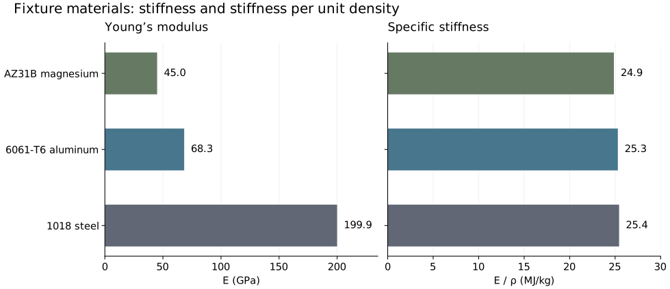
| Material | E (GPa) | ρ (Mg/m³) | E/ρ (MJ/kg) | Property source |
|---|---|---|---|---|
| AZ31B magnesium | 45.0 | 1.81 | 24.9 | ALLITE alloy comparison |
| 6061-T6 aluminum | 68.3 | 2.70 | 25.3 | Kaiser, pp. 2–3 |
| 1018 steel | 199.9 | 7.86 | 25.4 | Online Metals product guide |
The 6061-T6 entry uses the metric values printed in Kaiser’s table. The 1018 values are converted from 29,000 ksi and 0.284 lb/in³ before calculating the ratio; displayed values are rounded. Nominal values vary between references and product conditions.
For an ideal uniform beam, bending natural frequencies scale with √(E/ρ) when geometry and boundary conditions are fixed and the beam carries only its own distributed mass. The three materials give similar frequencies in this model. A fixture with an attached test item or flexible joints requires a model of the combined assembly.
At the same dimensions, steel provides a higher elastic bending stiffness EI and also contributes more moving mass. For a rectangular section, I = bh³/12, so bending stiffness varies with the cube of thickness h at fixed width b and modulus E. A lower-density material can permit a thicker section within a fixed mass budget. Check each material against the fixture geometry, payload, joint stiffness, strength requirements, and shaker limits.
Property inputs and calculated ratios (CSV) · Calculation and figure script (Python)
Baseline and low-level checks
Before full-level exposure, check mounting, cable clearance, channel orientation, sensor sensitivity, and the configured abort limits. A low-level run can reveal wiring errors, unexpected response peaks, and control problems. When comparing a shaker or fixture survey with a baseline, use the same documented configuration. A bare-table resonance frequency is specific to the shaker and setup.
Check required displacement against available travel before running the profile. Use the equipment manufacturer's approved verification procedure for travel checks. A low-level survey does not establish that the assembly will remain linear or within limits at the full test level.
4. Test types and excitation profiles
Sine sweeps and sweep duration
A sine test applies a periodic input. A sweep changes its frequency through a specified range; a dwell maintains a selected frequency. The profile must state whether amplitude means peak, peak-to-peak, or root mean square (RMS).
A linear sweep advances at a constant rate in Hz per unit time. A logarithmic sweep advances at a constant rate in octaves or decades per unit time. One octave doubles frequency. At a fixed octave rate, each frequency doubling takes the same time. Sweep speed affects the measured response near resonance because the vibration response takes time to build up and decay. Vibration Research: sweep range and sweep rate.
For a logarithmic sweep at R octaves per minute, the one-way duration is:
t = log₂(fhigh/flow) / R
Calculated example: 10 to 640 Hz spans six octaves. At 2 octaves per minute, one pass takes 3 minutes. An up-and-back cycle takes 6 minutes, excluding any pauses or ramps. State the number of passes and their directions; “cycle” can refer to either one pass or an up-and-back sweep.
Random vibration and power spectral density
Random vibration is described statistically. An acceleration power spectral density (PSD), commonly expressed in g²/Hz, specifies the distribution of mean-square acceleration across frequency. For a zero-mean signal and a one-sided PSD Ga(f), the overall RMS acceleration is:
aRMS = √[∫ Ga(f) df]
The integral uses frequency in Hz. On a logarithmic plot, the area drawn on the screen is not the integral. Two spectra can have the same RMS acceleration while distributing it across different frequencies. Their structural responses can differ. Vibration Research: random vibration and PSD.
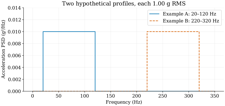
For a linear system with acceleration transfer function H(f), the response PSD is |H(f)|²Ginput(f). Input near a response peak is amplified more than input where |H(f)| is small. Overall input RMS alone does not describe response or fatigue exposure.
Mixed-mode excitation
Sine-on-random adds discrete tones to a broadband random background. Random-on-random adds narrow random bands to that background. Depending on the procedure, those tones or bands may remain fixed or sweep. Their levels and frequency schedules are separate parts of the test definition. Data Physics: mixed-mode control.
Mechanical shock and shock response spectrum
A mechanical shock is a transient input. A classical pulse, such as a half-sine pulse, is described in the time domain by its shape, amplitude, and duration. A shock response spectrum (SRS) reports the peak responses of a set of single-degree-of-freedom oscillators subjected to that input. Each oscillator has a specified natural frequency and damping.
State the damping and response convention used to calculate an SRS. Different time histories can produce similar SRS curves, so the spectrum does not uniquely identify the original waveform. An SRS calculated for one acceleration channel also does not specify a multi-axis test. Spectral Dynamics: shock response spectrum.
5. Test workflow and standards
Sequence for a documented test
- Define the exposure. Identify the governing requirement, test item configuration, mounting condition, axes, profile, duration, tolerances, and acceptance criteria.
- Mount and instrument. Record fixture and fastener details, sensor locations, channel roles, and pre-test functional results.
- Check at low level. Perform the required survey or equalization run. Review measured input and response, channel scaling, and limits before proceeding.
- Run the specified exposure. Follow the approved ramp and duration. Monitor control and response channels, operating function, and configured limits. Record interruptions and deviations.
- Inspect and compare. Perform the required post-test inspection and functional checks. If a repeat survey is specified, compare it with the baseline under the same mounting and acquisition conditions.
Follow the governing procedure for the required checks, their sequence, and the exposure duration.
Standards and test requirements
A standard name alone does not define a complete test. Record the required revision, method or section, applicable category, and approved tailoring. The following documents cover different applications:
- MIL-STD-810 includes vibration in Method 514 and shock in Method 516. Test conditions are tailored to the relevant service environment.
- RTCA DO-160 addresses environmental tests for airborne equipment. Section 8 covers vibration; Section 7 covers operational shocks and crash safety. Select the category for the specified installation.
- IEC 60068 includes sinusoidal vibration in Part 2-6 and broadband random vibration in Part 2-64.
- ISO 16750-3 covers mechanical loads for road-vehicle electrical and electronic equipment.
Use the applicable standard and approved test plan to determine the product’s profile and acceptance criteria.
Response limits and notching
Notching reduces the commanded input over selected frequency bands to keep a measured response or force within a specified limit. Document the basis for the limit and the resulting change to the exposure. A resonance alone does not justify a notch. MIL-HDBK-340A: force and response limiting.
Record the requested profile, achieved control spectrum, relevant response channels, and any active limits. Include deviations and interruptions in the exposure record.
What to record for a test
| Record | Information to retain |
|---|---|
| Requirement | Applicable document and revision, selected profile, axis, duration, and acceptance criteria. |
| Test item | Serial number, configuration, operating state, and pre-test functional results. |
| Mounting | Fixture identity, fasteners, specified torque, mounting orientation, and photographs. |
| Instrumentation | Sensor locations and orientations, calibration values, channel roles, and acquisition settings. |
| Exposure | Requested and achieved levels, elapsed time, limits, notches, aborts, and restarts. |
| Outcome | Observed damage, functional checks, deviations, and disposition against the stated acceptance criteria. |
The approved test procedure determines the required profile, tolerances, operating conditions, and pass/fail criteria. A test result applies to the documented configuration and exposure.
6. Signal analysis and quality metrics
Sampling and spectral measurements
The sample rate determines the Nyquist frequency, fs/2. An anti-alias filter must attenuate content that would fold into the measured band. For N acquired samples, the nominal record duration is N/fs and fast Fourier transform (FFT) bin spacing is:
Δf = fs/N = 1/T
Calculated example: 4,096 samples acquired at 2,048 samples/s form a 2-second record with 0.5 Hz bin spacing. A window changes leakage and the effective bandwidth of the spectral estimate. Zero padding gives more plotted frequency points but does not add information to the acquired record. NI: FFTs and windowing.
Retain the sample rate, record length, window, averaging method, and channel calibration with exported spectra. Those settings are needed to compare spectra between tests.
PSD estimation
A PSD estimate requires consistent FFT normalization, sample rate, window scaling, and one-sided or two-sided treatment. Squaring raw FFT values and dividing by a frequency interval is insufficient unless those conventions are also accounted for. Check the integral of the reported one-sided PSD against the mean-square value of the conditioned signal. Account for the estimator and finite record when comparing the two.
Frequency-bin spacing and effective spectral resolution are different quantities. Window bandwidth and averaging affect the estimate. Keep the same analysis settings when comparing runs, or account for the differences before interpreting a changed peak.
Frequency response functions and coherence
A frequency response function (FRF) describes a complex response-to-input relationship, including magnitude and phase. Its units depend on the channels: acceleration divided by force is accelerance, whereas acceleration divided by base acceleration is dimensionless transmissibility. Accelerance relates response to applied force; transmissibility relates response to base motion.
Magnitude-squared coherence is commonly written γ²(f) = |Gxy(f)|²/[Gxx(f)Gyy(f)], using averaged cross- and autospectra. Values range from zero to one. Low coherence can result from noise, unmeasured inputs, leakage, nonlinear response, or changing conditions. High coherence supports a consistent linear relationship in that measurement; it does not by itself prove causation or verify the sensor calibration. NI: frequency-response and coherence analysis.
Random peaks and kurtosis
A random waveform need not have a Gaussian amplitude distribution. Pearson kurtosis is the fourth central moment divided by the square of the variance. A Gaussian distribution has kurtosis 3; the alternative excess-kurtosis convention subtracts 3 and therefore gives zero. State which convention is used.
Kurtosis control can alter the amplitude distribution while retaining a target PSD and RMS level. Signals with equal PSD and RMS can have different peak statistics. A chosen kurtosis also does not uniquely specify a waveform or demonstrate equivalent fatigue damage. Vibration Research: kurtosis control.
Sources and calculation files
Prepared from my vibration-testing study notes, with the manufacturer and NASA references linked above. The figures show calculated examples. Licensed DO-160 profile tables and customer test profiles are not reproduced.
Calculated example values (JSON) · Figure-generation script (Python)